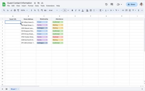
Applying Alternating Row Colors in Google Sheets
You can easily color every other row using Google Sheets' built-in "Alternating colors" feature. This formatting is dynamic, meaning it will adjust automatically if you insert or delete rows within the formatted range.
Follow these steps:
- Select the Range: Click and drag to highlight the cells or entire rows you want to format. To select the whole sheet, click the empty rectangle in the top-left corner (above row 1 and to the left of column A).
- Access Format Options: Go to the main menu and click on Format.
- Apply Alternating Colors: From the dropdown menu, choose Alternating colors. A sidebar will open on the right.
- Customize Appearance (Optional): In the "Alternating colors" sidebar, you can:
- Choose from predefined Styles.
- Specify if your selection includes a Header or Footer for separate formatting by checking the respective boxes.
- Select custom colors for Color 1 (primary rows) and Color 2 (alternating rows).
- To remove the formatting later, ensure the previously formatted range is selected, then click "Remove alternating colors" at the bottom of this sidebar. If the sidebar is not open, select the range and go to Format > Alternating colors to reopen it.