To color every other row in Google Sheets, you can use the "Alternating colors" feature or a custom formula.
Method 1: Using Alternating Colors
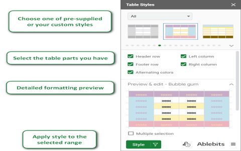
- Select the range of cells you want to apply the formatting to.
- Go to Format > Alternating colors.
- A sidebar will appear. Choose your desired style, including header/footer rows and color scheme.
- Click Done.
Method 2: Using a Custom Formula
- Select the range of cells you want to apply the formatting to.
- Go to Format > Conditional formatting.
- In the "Apply to range" field, ensure your desired range is selected.
- Under "Format rules", in the "Format cells if" dropdown, select "Custom formula is".
- Enter one of the following formulas:
- To color even rows:
=ISEVEN(ROW()) - To color odd rows:
=ISODD(ROW())
- To color even rows:
- Choose the desired background color.
- Click Done.
Explanation of the formulas:
ROW()returns the row number of the current cell.ISEVEN()returns TRUE if the row number is even, and FALSE otherwise.ISODD()returns TRUE if the row number is odd, and FALSE otherwise.